Differential Algebraic Machine Learning in Linear PDE Solution Spaces
SCML 2026: International Conference on Symbolic Computation and Machine Learning, SCDDE 2026: Symbolic Computation and Differential and Difference Equations
Markus Lange-Hegermann



With many, many contributions by Obed Amo, Andreas Besginow, Samit Ghosh, Marc Härkönen, Jianlei Huang, Xin Li, Michael Pokojovy, Bogdan Raiță, Daniel Robertz, and Jörn Tebbe






Thx for having me!
A personal Motivation
What about Data and Functions?
- describe analytic system behavior ($\rightarrow$ functional analysis) nor
- account for (noisy) data ($\rightarrow$ stochastics, machine learning)
Goal:
Data structures for $\mathcal{F}$ that...- can be trained to approximate any function in $\textcolor{FF9700}{\mathcal{F}^{m_0}}$,
- incorporates a probability distribution on $\textcolor{FF9700}{\mathcal{F}^{m_0}}$, or
- is compatible to techniques in algebra, functional analysis, stochastics, and/or machine learning.
Example
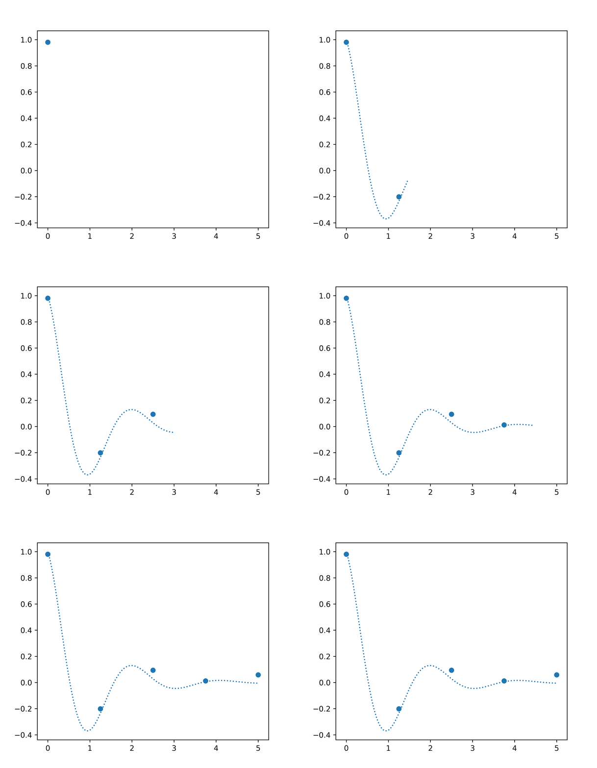
Damped spring-mass system
\[\frac{\mathrm{d}^2y}{\mathrm{d}t^2} + 2 \frac{\mathrm{d}y}{\mathrm{d}t} + 10y = 0\] Sample 5 noisy points
Example
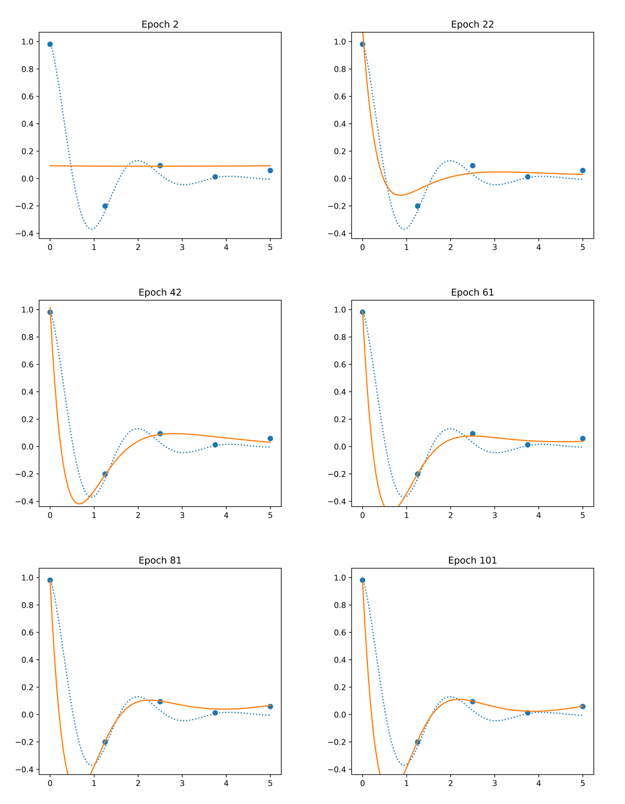
Neural Network
- ⚠️ ~300,000 parameters
- ✅ Fast convergence
- ❌ Bad inter/extrapolation
Example
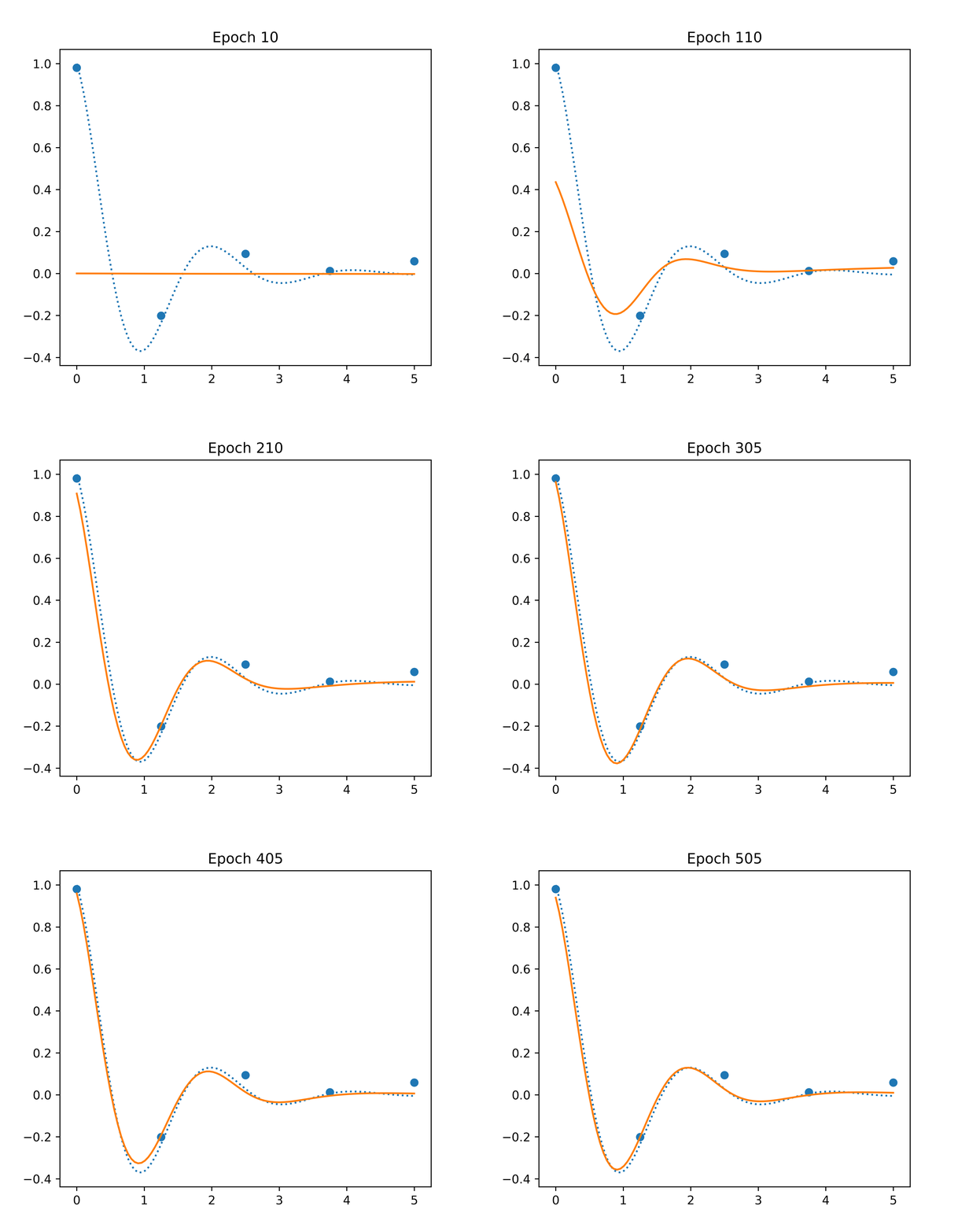
Physics Informed Neural Network
- ✅ Good interpolation
- ✅ Fast inference
- ⚠️ ~300,000 parameters
- ⚠️ Requires extra points
- ⚠️ Not an exact solution
- ❌ Slow convergence
- ❌ Hard to optimize
A more constrained approach
How would you solve?
\[\frac{\mathrm{d}^2y}{\mathrm{d}t^2} + 2 \frac{\mathrm{d}y}{\mathrm{d}t} + 10y = 0\]
Algebraic preprocessing: characteristic frequencies \[z^2 + 2z + 10 = 0 \Rightarrow z = -1 \pm 3\sqrt{-1}\]
Solution Space \[y(t) = (\textcolor{#b51963}{c_1} \cdot e^{-t} \cos 3t + \textcolor{#b51963}{c_2} \cdot e^{-t} \sin 3t)\]
A more constrained approach
\[\frac{\mathrm{d}^2y}{\mathrm{d}t^2} + 2 \frac{\mathrm{d}y}{\mathrm{d}t} + 10y = 0\]
Algebraic preprocessing: characteristic frequencies \[z^2 + 2z + 10 = 0 \Rightarrow z = -1 \pm 3\sqrt{-1}\]
Solution Space \[y(t) = (\textcolor{#b51963}{c_1} \cdot e^{-t} \cos 3t + \textcolor{#b51963}{c_2} \cdot e^{-t} \sin 3t)\]
Algebra: determine suitable frequencies
Stochastics: weigh frequencies
A more constrained approach
\[\frac{\mathrm{d}^2y}{\mathrm{d}t^2} + 2 \frac{\mathrm{d}y}{\mathrm{d}t} + 10y = 0\]
Algebraic preprocessing: characteristic frequencies \[z^2 + 2z + 10 = 0 \Rightarrow z = -1 \pm 3\sqrt{-1}\]
Solution Space \[y(t) = (\textcolor{#b51963}{c_1} \cdot e^{-t} \cos 3t + \textcolor{#b51963}{c_2} \cdot e^{-t} \sin 3t)\]
Algebra: determine suitable frequencies
Stochastics: weigh frequencies
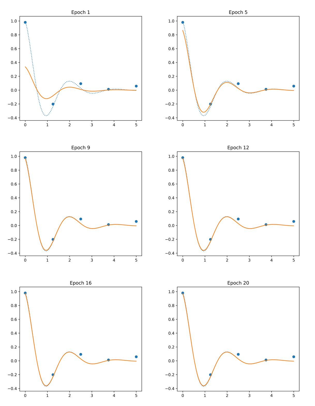
Gaussian process prior \[Y(t) \sim (\textcolor{#b51963}{C_1} \cdot e^{-t} \cos 3t + \textcolor{#b51963}{C_2} \cdot e^{-t} \sin 3t) + \textcolor{#b51963}{\epsilon}\] where \[ \textcolor{#b51963}{C_1 \sim \mathcal{N}(0, \sigma_1^2)}, \textcolor{#b51963}{C_2 \sim \mathcal{N}(0, \sigma_2^2)}, \textcolor{#b51963}{\epsilon \sim \mathcal{N}(0, \sigma_0^2)} \]
Gaussian Process
- ✅ 3 parameters
- ✅ Fast convergence
- ✅ Good inter/extrapolation
- ✅ Exact solution
- ✅ No extra points
Gaussian Processes
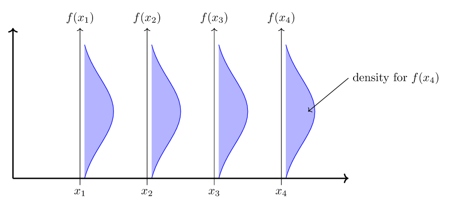
Assume Gaussian function values of the regression function $f$.
Gaussian Processes
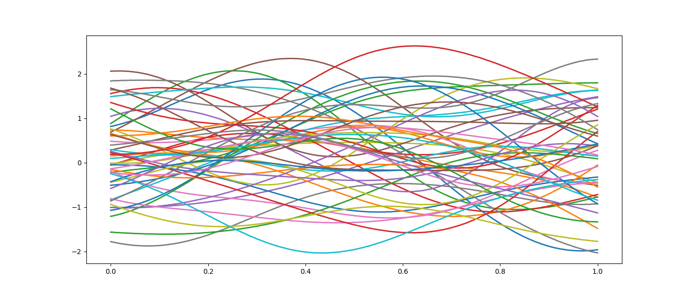
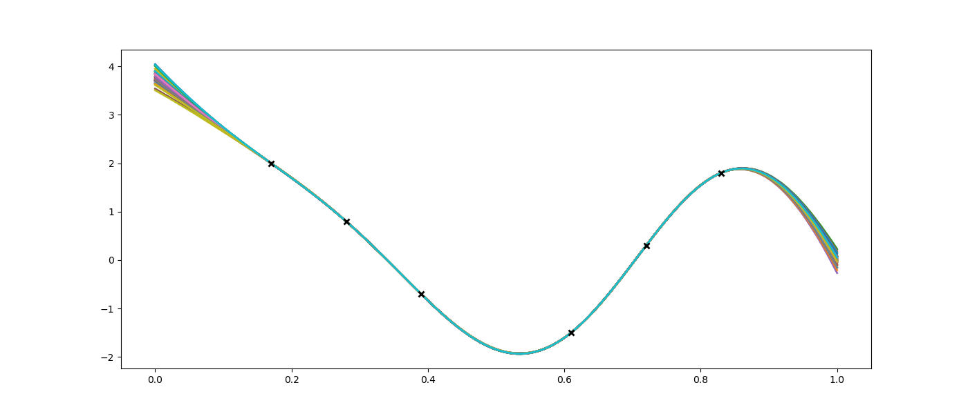
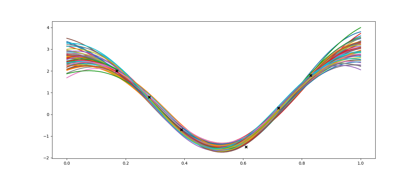
Characterizing GPs
| Gaussian distribution $1$-dim | Gaussian distribution $n$-dim | GPs |
|---|---|---|
| $\textcolor{b51963}{\mathcal{N}(\mu,\sigma^2)}$ | $\textcolor{b51963}{\mathcal{N}(\mu,\Sigma)}$ | $\textcolor{b51963}{\mathcal{GP}(\mu(x),k(x_1,x_2))}$ |
| Mean $\textcolor{b51963}{\mu}$ | Mean vector $\textcolor{b51963}{\mu}$ | Mean function $\textcolor{b51963}{\mu}$ |
| Variance $\textcolor{b51963}{\sigma^2}$ | Covariance matrix $\textcolor{b51963}{\Sigma}$ | Covariance function $\textcolor{b51963}{k}$ |
GPs
GPs
GPs
Encoding knowledge into GPs
Smith Normal Form
there are invertible matrices $S$ and $\textcolor{#0073e6}{T}$ s.t. \[ \begin{align*} SA\textcolor{#0073e6}{T}=D \end{align*} \] where $D$ is a diagonal matrix.
Smith Normal Form
| $h_1(t)=0$ | $k_1(t_1,t_2)=0$ | |
| $h_2(t)=\textcolor{#b51963}{c_1}\sin(t)+\textcolor{#b51963}{c_2}\cos(t)$ | $\textcolor{#b51963}{c_1,c_2\sim\mathcal{N}(0,\sigma^2)}$ | $k_2(t_1,t_2)=\textcolor{#b51963}{\sigma^2}\cos(t_1-t_2)$ |
| $h_3(t)$ arbitrary | $\text{\textcolor{#b51963}{Smooth prior}}$ | $k_3(t_1,t_2)=\exp(-\frac{1}{2}(t_1-t_2)^2)$ |
Smith Normal Form
| $h_1(t)=0$ | $k_1(t_1,t_2)=0$ | |
| $h_2(t)=\textcolor{#b51963}{c_1}\sin(t)+\textcolor{#b51963}{c_2}\cos(t)$ | $\textcolor{#b51963}{c_1,c_2\sim\mathcal{N}(0,\sigma^2)}$ | $k_2(t_1,t_2)=\textcolor{#b51963}{\sigma^2}\cos(t_1-t_2)$ |
| $h_3(t)$ arbitrary | $\text{\textcolor{#b51963}{Smooth prior}}$ | $k_3(t_1,t_2)=\exp(-\frac{1}{2}(t_1-t_2)^2)$ |
Theorem: The resulting set of realizations is $C^\infty$-dense in $\operatorname{sol}_\mathcal{F}(A)$.
Optimal Control
Example: HMC sampling for constrained control
$ \dot{\begin{pmatrix} \textcolor{1F77B4}{x_1} \\ \textcolor{FF7F0E}{x_2} \end{pmatrix}} = \begin{pmatrix} 0 & 1 \\ -1 & 0 \end{pmatrix} \begin{pmatrix} \textcolor{1F77B4}{x_1} \\ \textcolor{FF7F0E}{x_2} \end{pmatrix} + \begin{pmatrix} 0 \\ 1 \end{pmatrix} \textcolor{2CA02C}{u} $
Rougher Covariance (GPM) with energy reduction bias (GPMO)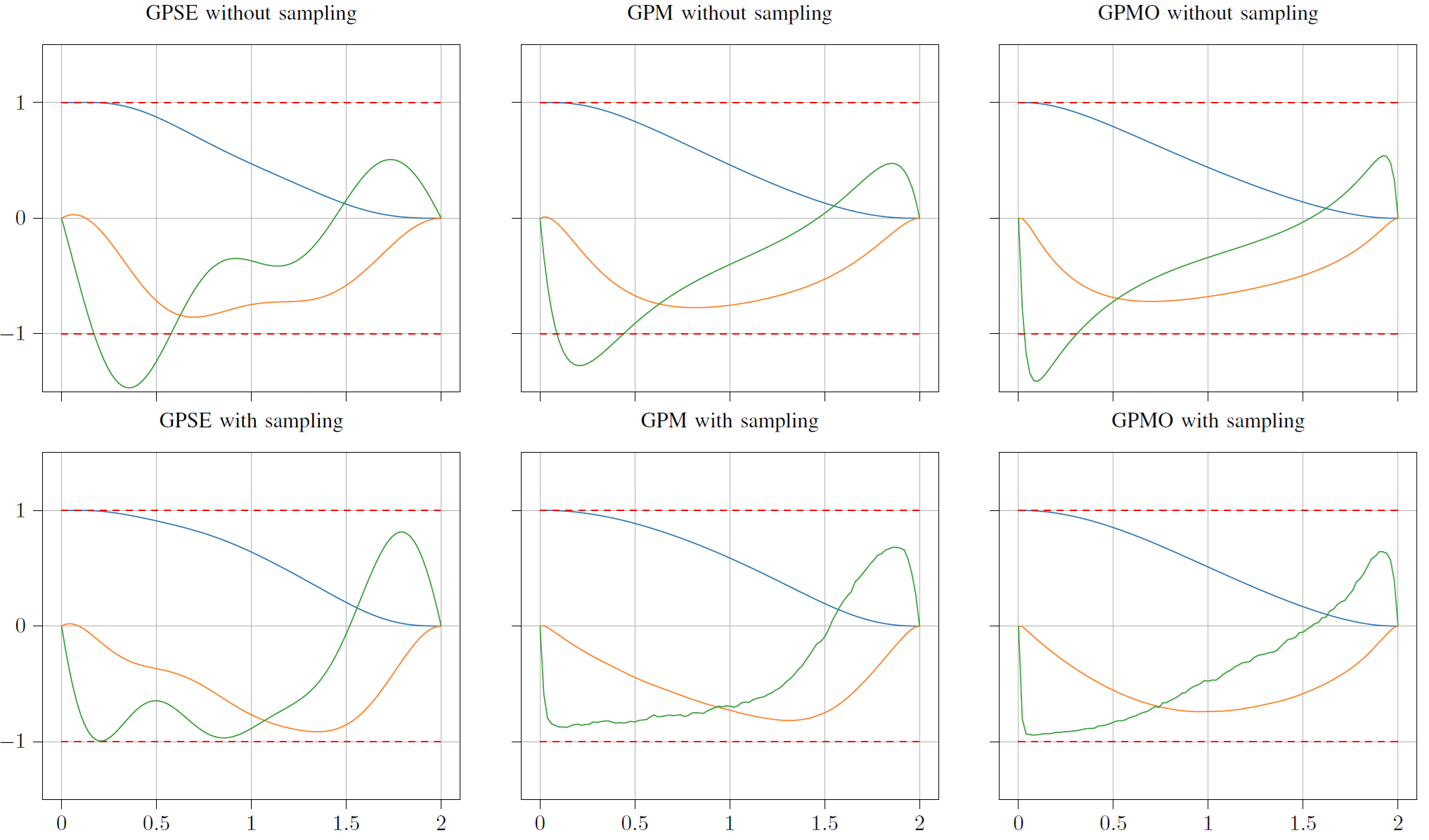
Example: HMC sampling for constrained control
$ \dot{\begin{pmatrix} \textcolor{1F77B4}{x_1} \\ \textcolor{FF7F0E}{x_2} \end{pmatrix}} = \begin{pmatrix} 0 & 1 \\ 0 & 0 \end{pmatrix} \begin{pmatrix} \textcolor{1F77B4}{x_1} \\ \textcolor{FF7F0E}{x_2} \end{pmatrix} + \begin{pmatrix} 0 \\ 1 \end{pmatrix} \textcolor{2CA02C}{u} $
Rougher Covariance (GPM) with energy reduction bias (GPMO)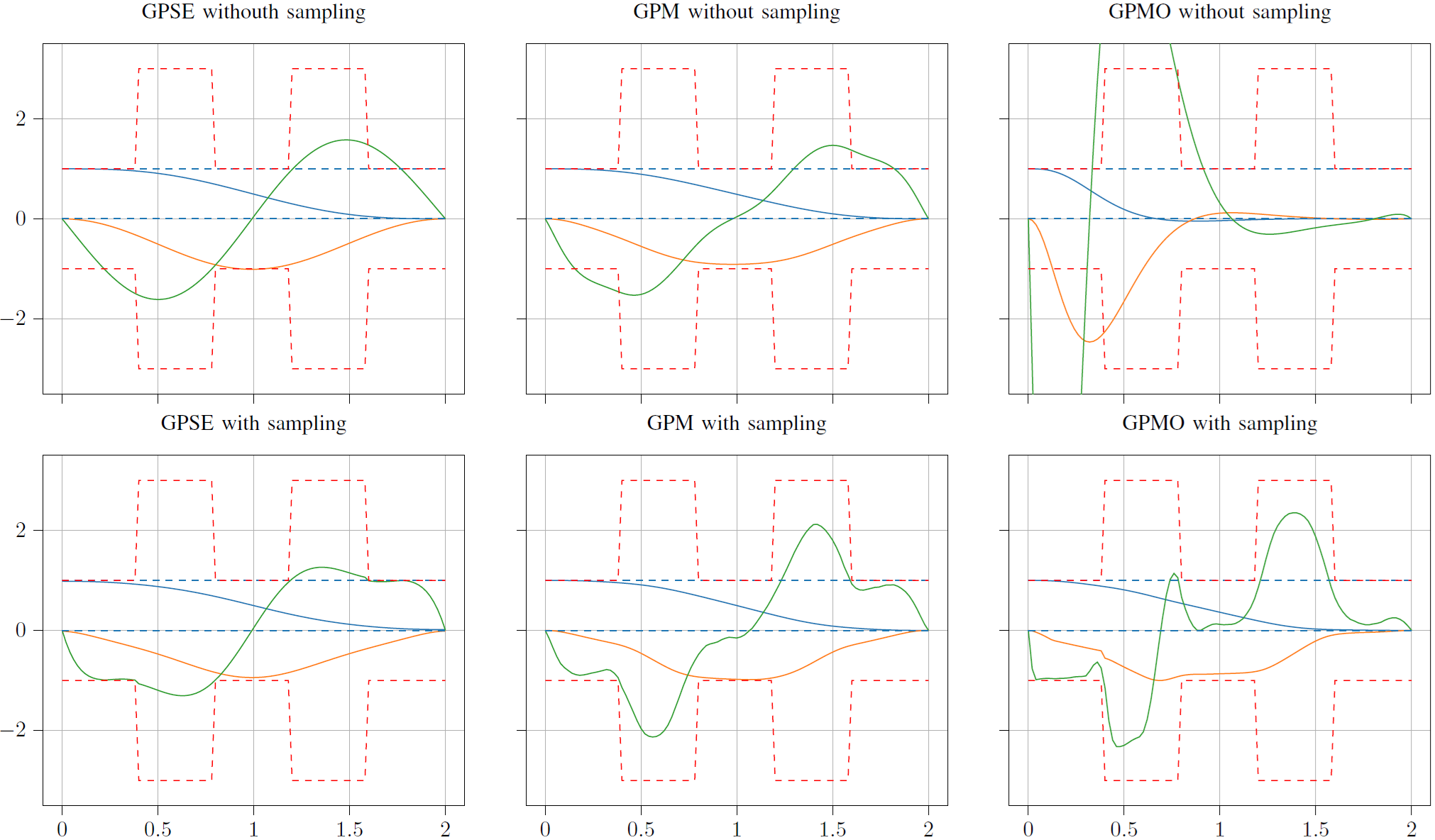
PDEs
You cannot solve PDEs with data, solutions are rarely unique!
Cosinder regression in the solution space.
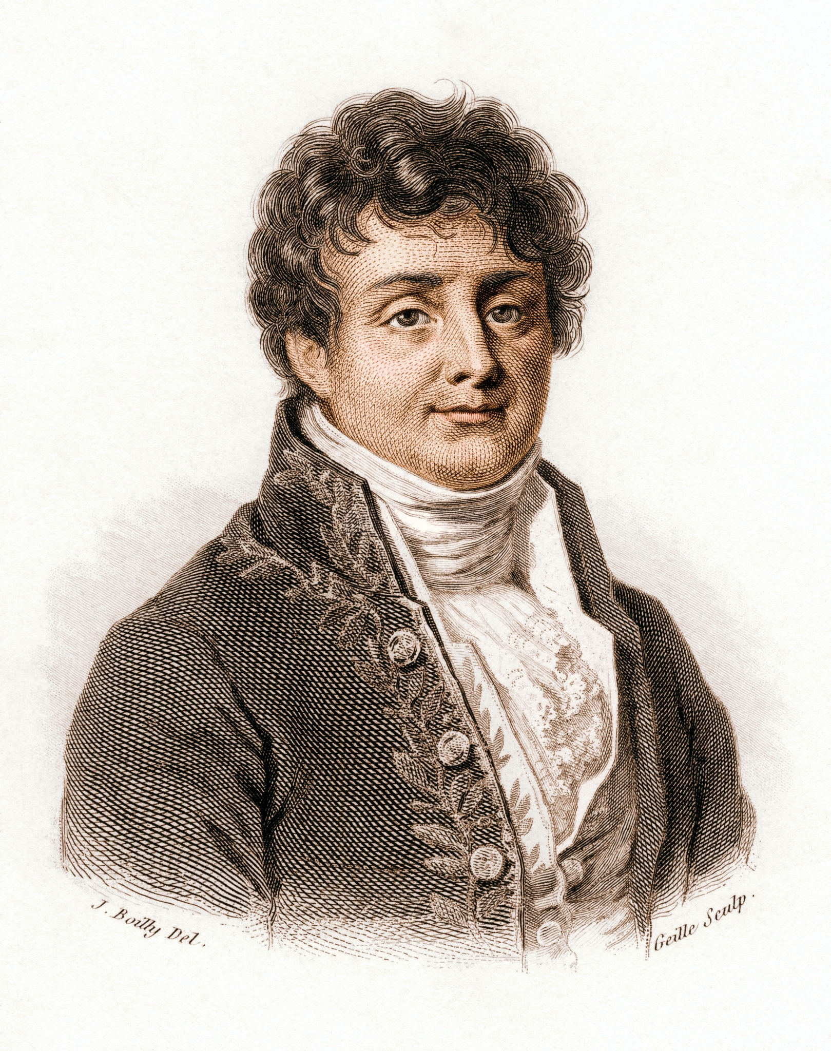
Fourier & Heat Equation (1822)
\[\frac{\partial T}{\partial t}-\frac{\partial^2 T}{\partial x^2}=0\]
- $e^{\textcolor{#0073e6}{-z^2}t+\textcolor{#0073e6}{\sqrt{-1}z}x}=e^{-z^2t}(\cos zx+\sqrt{-1}\sin zx)$ are solutions.
- Linearity: $T^c(x,z)=\sum_{z=-N}^N \textcolor{#b51963}{c_z}e^{\textcolor{#0073e6}{-z^2}t+\textcolor{#0073e6}{\sqrt{-1}z}x}$ are solutions.
- Postulated density: All solutions $T$ can be approximated with solutions $T^c$.
- Considered initial conditions $T^c(x,0)=\sum_{z\in\mathbb Z} \textcolor{#b51963}{c_z}e^{\textcolor{#0073e6}{\sqrt{-1}z}x}$ (Fourier series).
Ehrenpreis-Palamodov (1970)
Solutions to a linear PDE system $Af=0$ with constant coefficients are described by Fourier frequencies
\[ f(x) = \int_{\textcolor{#0073e6}{V}} \textcolor{#0073e6}{B(x,z)} e^{\langle x, \textcolor{#0073e6}{z} \rangle} \, \mathrm{d}\textcolor{#b51963}{\mu(z)} \] Algebraic preprocessing Learned
- $V$ encodes frequencies
- $B$ encodes multiplicity of frequencies and dependencies between outputs
- $\mu(z)$ weighs frequencies
Ehrenpreis-Palamodov (1970)
Let $A \in R^{\ell' \times {\ell}}$ for $R=\R[\partial_{x_1},\ldots,\partial_{x_n}]$ and let $\Omega \subseteq \R^n$ be a convex, compact set. There exist
- characteristic varieties $\textcolor{#0073e6}{\{V_1,\dotsc,V_s\}}$ and
- $\ell\times1$ polynomial operators $\textcolor{#0073e6}{\{B_{i,1}(x, z), \dotsc, B_{i,m_i}(x,z)\}_{i=1,\dotsc,s}}$ in $2n$ variables,
such that any smooth solution $f \colon \Omega \to \R^{\ell}$ to the equation $Af = 0$ can be written as \[ \begin{align*} f(x) &= \sum_{i=1}^s \sum_{j=1}^{m_i} \int_{\textcolor{#0073e6}{V_i}} \textcolor{#0073e6}{B_{i,j}(x, z)} e^{\langle x, \textcolor{#0073e6}{z} \rangle} \textcolor{#b51963}{\mathrm{d}\mu_{i,j}(z)} \end{align*} \] for a suitable choice of measures $\textcolor{#b51963}{\mu_{i,j}}$.
Compute associated primes $V_i$ of the system module of $A$.
When localizing at $V_i$, the $B_i$ are the parametrizations of $A$ (up to technical details).
EPGP
Combine the EP-representation for both $x, x'$ with a Gaussian measure for the frequencies $z$. \[ \begin{align*} \Psi(x,z) &:= \sum_j \textcolor{#0073e6}{B_j(x,z)} e^{\langle x, \textcolor{#0073e6}{z} \rangle} \\ k_{\operatorname{EPGP}}(x,x') &:= \int_{\sqrt{-1}z \in \textcolor{#0073e6}{V}} \Psi(x,z) \, \textcolor{#b51963}{e^{-\frac{\|z\|^2}{2}}}\, \Psi(x',z)^H \, \textcolor{#b51963}{\mathrm{d}z}. \end{align*} \] Imaginary frequencies yield a stationary covariance.
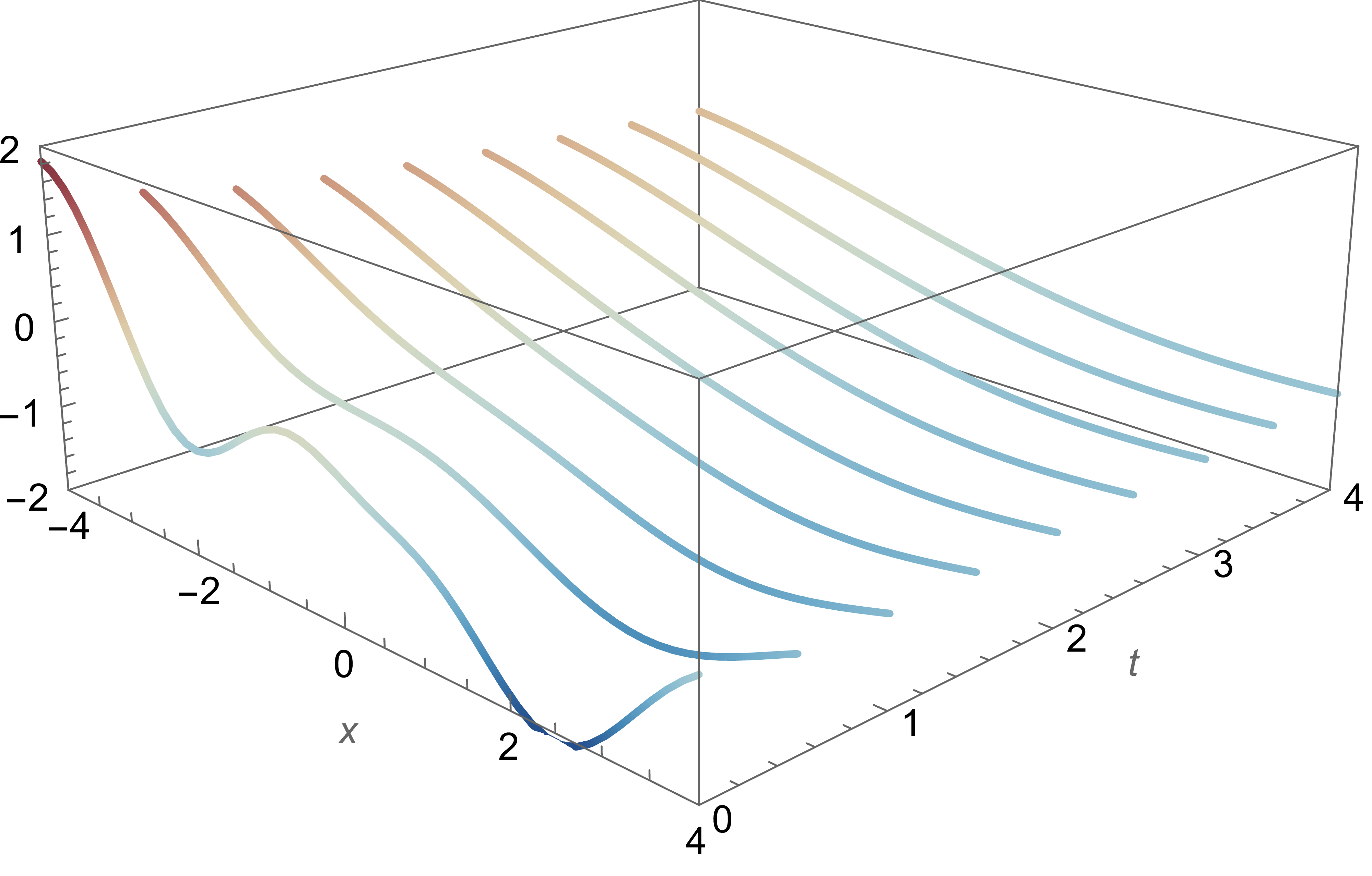
Heat Equation
Parametrize characteristic variety $\textcolor{#0073e6}{V( z_1^2 - z_2)}$ by $z_1=\sqrt{-1}z$ and $z_2=(\sqrt{-1}z)^2$ for $z\in\mathbb{R}$.
$\textcolor{#0073e6}{B=\begin{bmatrix}1\end{bmatrix}}$. \[ \begin{align*} k_\text{heat}(x,t;x',t') &= \int_{z \in \R} e^{\sqrt{-1}zx} e^{-z^2t} \textcolor{#b51963}{e^{-\frac{z^2}{2}}} e^{-z^2t'} e^{\overline{\sqrt{-1}}zx'} \, \textcolor{#b51963}{d\mathcal{L}(z)} \\ &= \sqrt{2\pi} \frac{e^{-\frac{(x-x')^2}{2(1+2(t+t'))}}}{\sqrt{1+2(t+t')}} \end{align*} \]
Heat Equation
Heat Equation
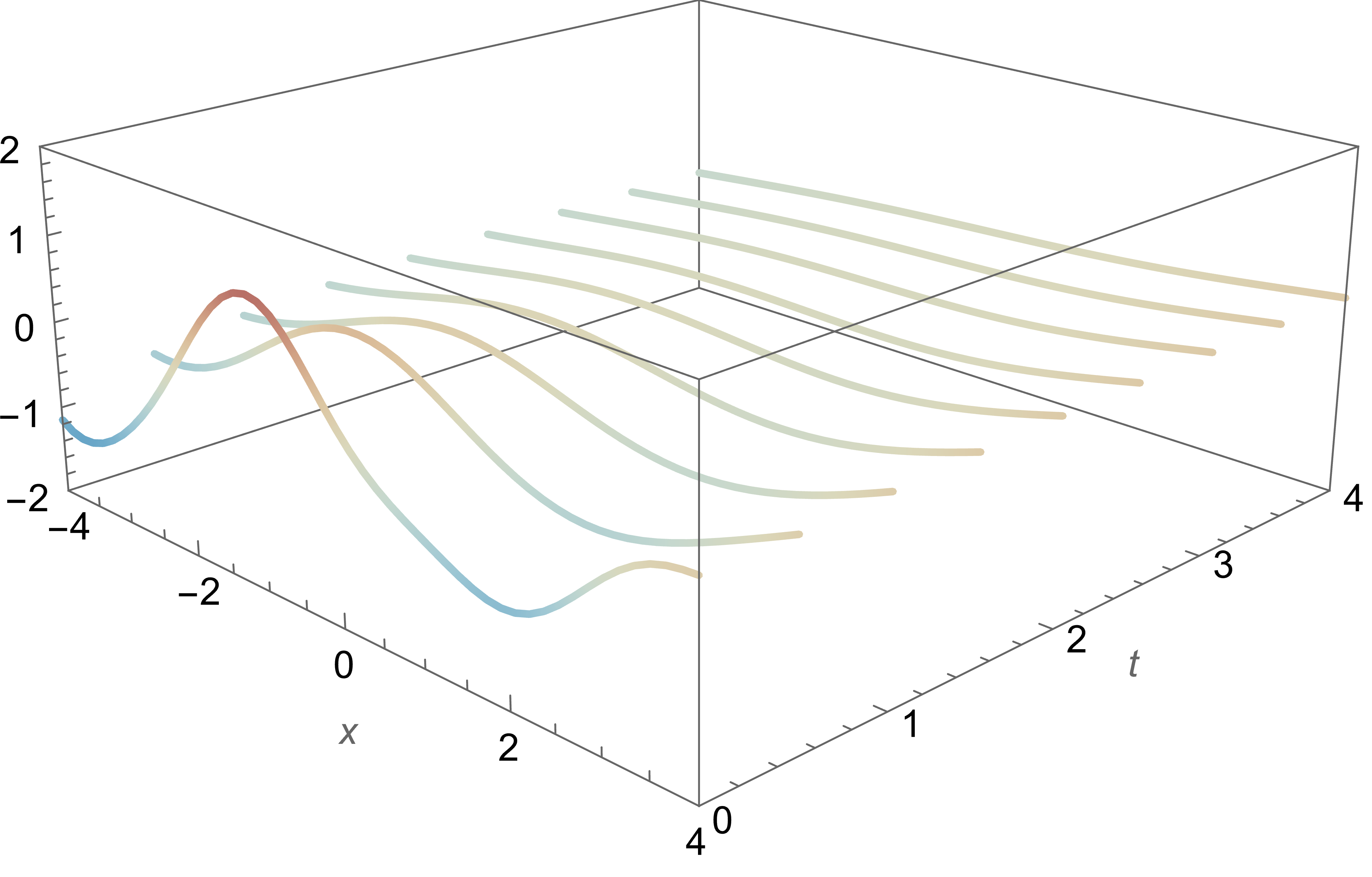
Heat Equation
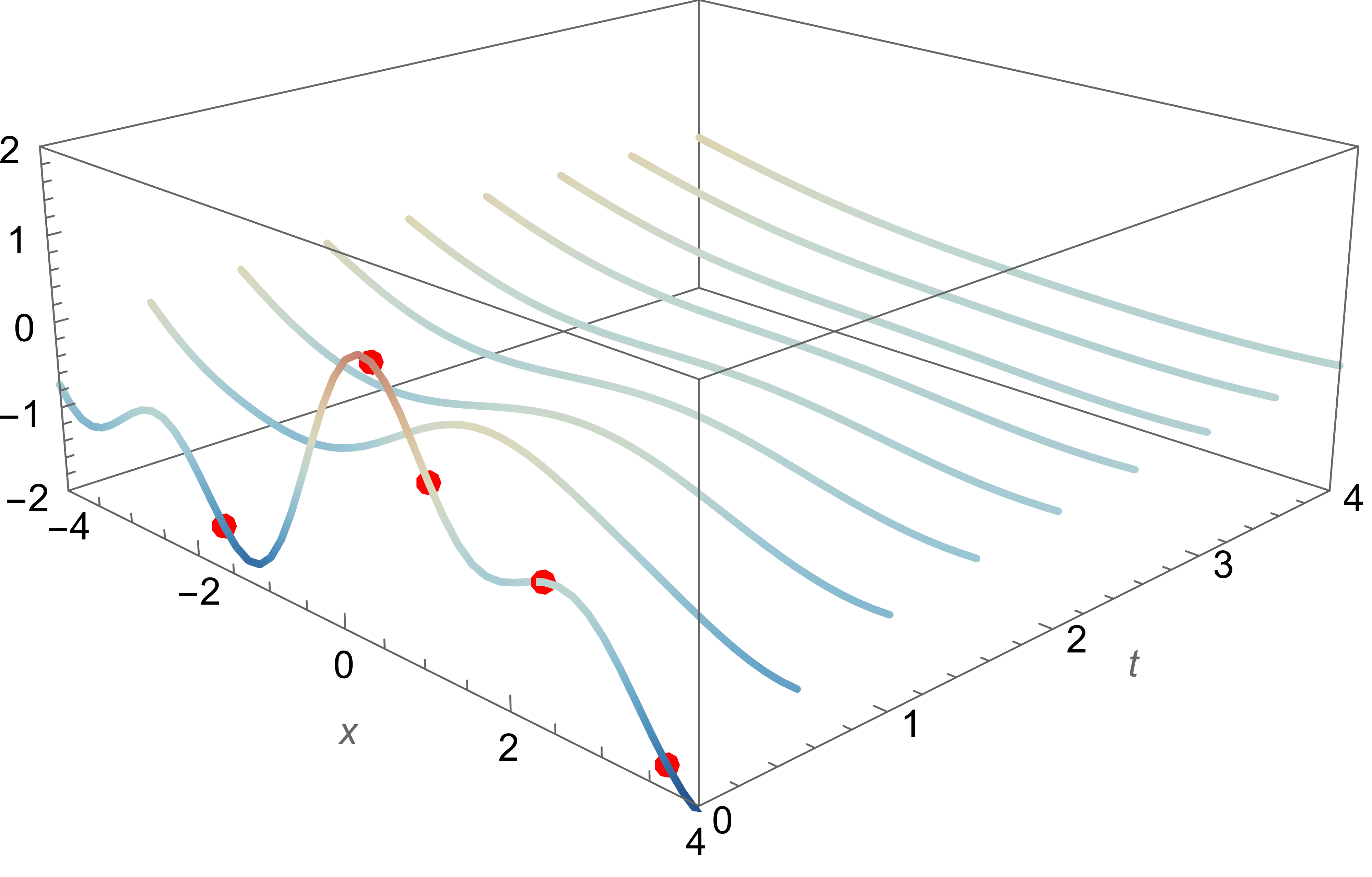
Heat Equation
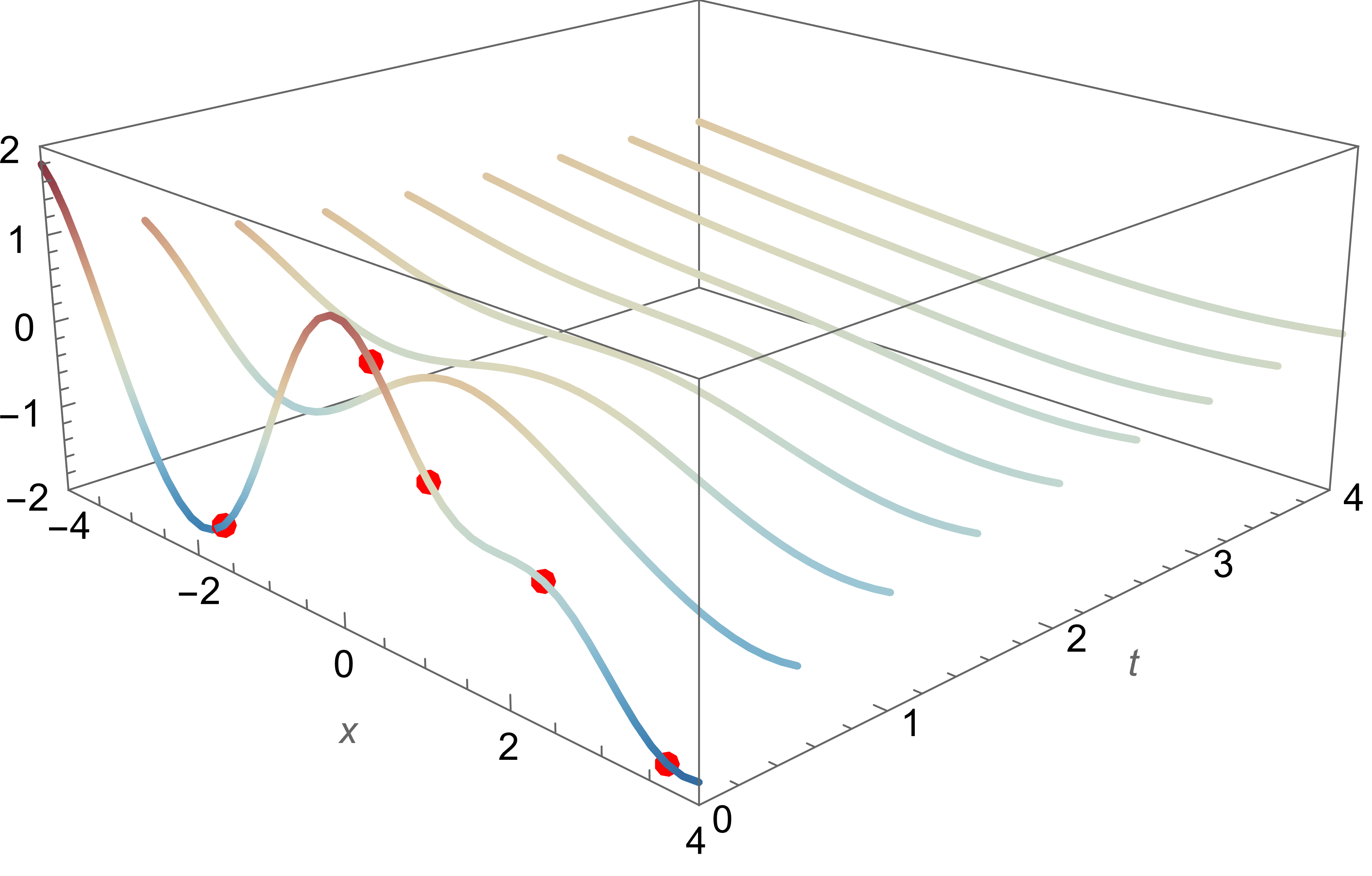
Heat Equation
Cuomo, Di Cola, Giampaolo, Rozza, Raissi, Piccialli; Scientific machine learning through physics-informed neural networks: Where we are and what’s next. Journal of Scientific Computing; arXiv:2201.05624
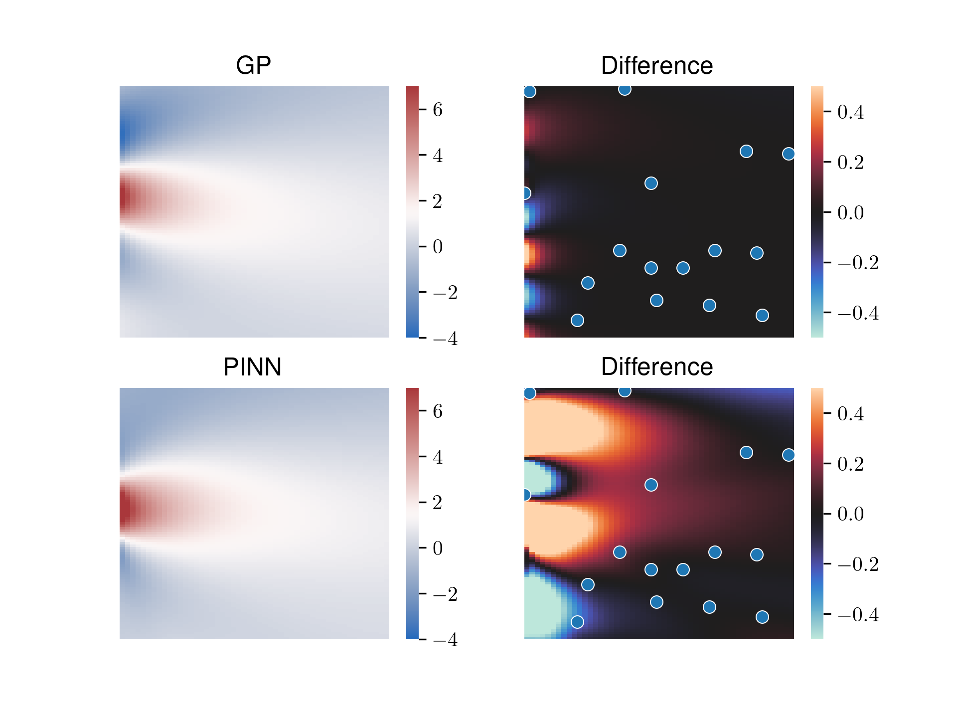
Heat Equation
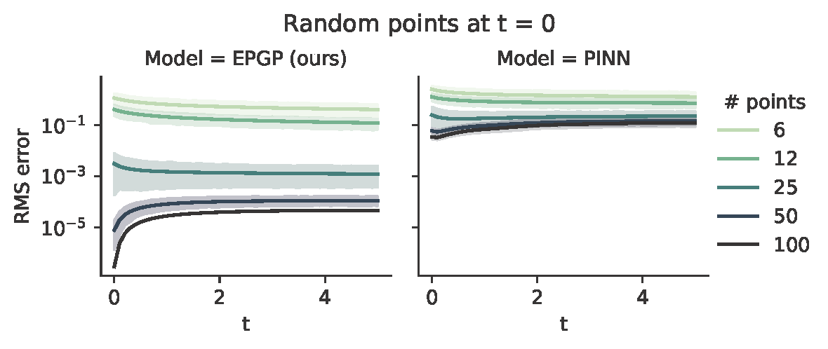
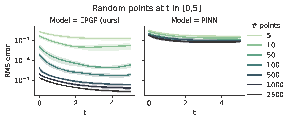
S-EPGP
Sparse version of EPGP without integration.
- Choose the measures $\textcolor{#b51963}{\mu_{i,j}}$ as linear combinations of trainable Dirac deltas at points $\textcolor{#0073e6}{z_{i,j} \in V}$.
- Define a GP prior with realizations of the form \[ \begin{align*} f(x) = \sum_{j=1}^m \sum_{i=1}^r \textcolor{#b51963}{c_{i,j}} \textcolor{#0073e6}{B_j}(x, \textcolor{#0073e6}{z_{i,j}}) e^{\langle x, \textcolor{#0073e6}{z_{i,j}} \rangle} =: \textcolor{#b51963}{c^T}\cdot \textcolor{#0073e6}{\phi(x)}, \end{align*} \]
- Turn $f(x)$ into a GP: $\textcolor{#b51963}{c_{i,j} \sim \mathcal{N}\left(0, \frac{1}{mr} \Sigma\right)}$ for $\textcolor{#b51963}{\Sigma=\operatorname{diag}(\sigma_{i}^2)}$
S-EPGP
Sparse version of EPGP without integration.
- Choose the measures $\textcolor{#b51963}{\mu_{i,j}}$ as linear combinations of trainable Dirac deltas at points $\textcolor{#0073e6}{z_{i,j} \in V}$.
- Define a GP prior with realizations of the form \[ \begin{align*} f(x) = \sum_{j=1}^m \sum_{i=1}^r \textcolor{#b51963}{c_{i,j}} \textcolor{#0073e6}{B_j}(x, \textcolor{#0073e6}{z_{i,j}}) e^{\langle x, \textcolor{#0073e6}{z_{i,j}} \rangle} =: \textcolor{#b51963}{c^T}\cdot \textcolor{#0073e6}{\phi(x)}, \end{align*} \]
- Turn $f(x)$ into a GP: $\textcolor{#b51963}{c_{i,j} \sim \mathcal{N}\left(0, \frac{1}{mr} \Sigma\right)}$ for $\textcolor{#b51963}{\Sigma=\operatorname{diag}(\sigma_{i}^2)}$
Wave equation 2D
\[\frac{\partial^2 u}{\partial t^2} = \frac{\partial^2 u}{\partial x^2} + \frac{\partial^2 u}{\partial y^2}\]
Wave equation 2D
\[\frac{\partial^2 u}{\partial t^2} = \frac{\partial^2 u}{\partial x^2} + \frac{\partial^2 u}{\partial y^2}\]
Numerical solution: Mean of our S-EPGP:
 PINN:
PINN:

Training data: spatial $21\times21$-grid of the first three frames of the numerical solution.
Wave equation 2D
\[\frac{\partial^2 u}{\partial t^2} = \frac{\partial^2 u}{\partial x^2} + \frac{\partial^2 u}{\partial y^2}\]
Wave equation 2D
\[\frac{\partial^2 u}{\partial t^2} = \frac{\partial^2 u}{\partial x^2} + \frac{\partial^2 u}{\partial y^2}\]
Boundary conditions B-EPGP
Homogeneous Maxwell's equations
\[\mathbf{E}(x,y,z,t)\]
3D wave equation
\[ \mathbf{B}(x,y,z,t) \]
Special case for PDEs: Various equivalent conditions
- Solution set allows for full frequency spectrum (harmonic analysis)
- System is controllable (engineering)
- Solution set admits potentials (physics)
- System module is torsionless (algebraic system theory)
- System module is reflexive (homological algebra)
- Solution set is parametrizable by a linear operator (functional analysis)
The Koszul (or de Rham) Complex
Parametrized by $\textcolor{#0073e6}{B=\begin{bmatrix} 0 & x_3 & -x_2 \\ -x_3 & 0 & x_1 \\x_2 & -x_1 & 0 \\\end{bmatrix}} $.
Covariance function for tangential fields on the sphere: \[ \begin{bmatrix} -y_1y_2-z_1z_2 & y_1x_2 & z_1x_2 \\ x_1y_2 & -x_1x_2-z_1z_2 & z_1y_2 \\ x_1z_2 & y_1z_2 & -x_1x_2-y_1y_2\\ \end{bmatrix}\cdot k \]
The Koszul (or de Rham) Complex
Parametrized by $\textcolor{#0073e6}{B=\begin{bmatrix} 0 & x_3 & -x_2 \\ -x_3 & 0 & x_1 \\x_2 & -x_1 & 0 \\\end{bmatrix}}$.
Covariance function for tangential fields on the sphere: \[ \begin{bmatrix} -y_1y_2-z_1z_2 & y_1x_2 & z_1x_2 \\ x_1y_2 & -x_1x_2-z_1z_2 & z_1y_2 \\ x_1z_2 & y_1z_2 & -x_1x_2-y_1y_2\\ \end{bmatrix}\cdot k \]

The Koszul (or de Rham) Complex
$\textcolor{#0073e6}{B=\begin{bmatrix} 0 & x_3 & -x_2 \\ -x_3 & 0 & x_1 \\x_2 & -x_1 & 0 \\\end{bmatrix}}$
via a pullback under suitable assumptions

The Koszul (or de Rham) Complex
via a pullback under suitable assumptions

The Koszul (or de Rham) Complex
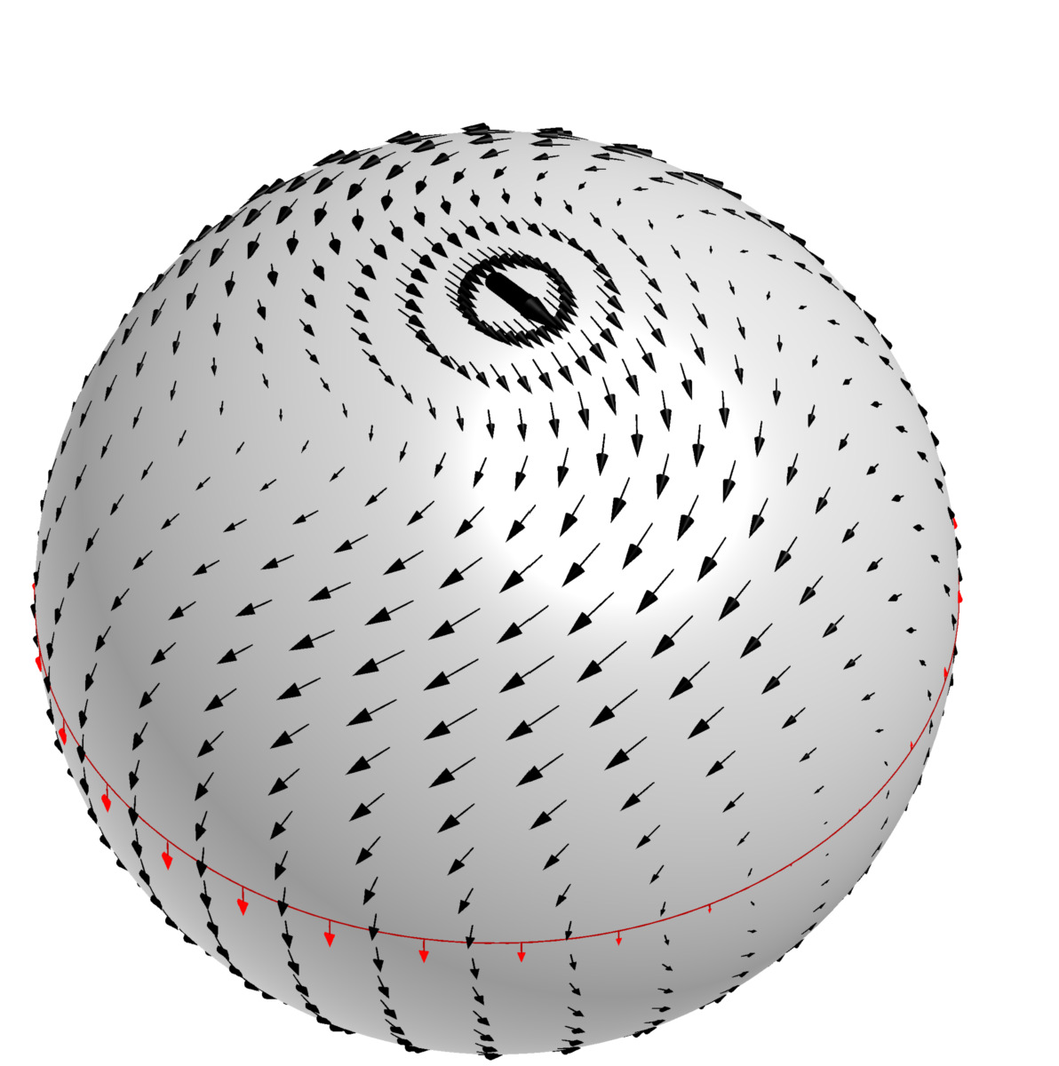
Smooth divergence free fields $f$ on the sphere and
inhomogeneous boundary condition $f_3(x_1,x_2,0)=x_2$.
Modeling with few data points
Modeling with many data points
- GPs suffer from $\mathcal{O}(\textcolor{#b51963}{\operatorname{data}^2})$ space complexity and $\mathcal{O}(\textcolor{#b51963}{\operatorname{data}^3})$ time complexity.
- Consider: $u(t,x)$ satisfying the transport equation $\begin{bmatrix}\partial_t-\partial_x\end{bmatrix}\cdot u(t,x)=0$.
- Ansatz: $u(t,x)=\sigma(z_1t+z_2x+b)$.
- Then $\begin{bmatrix}\partial_t-\partial_x\end{bmatrix}\cdot u(t,x)=0\Leftrightarrow\textcolor{#0073e6}{(z_1-z_2)}\cdot\sigma'(z_1t+z_2x+b)=0\Leftarrow \textcolor{#0073e6}{z_1=z_2}$.
- Hence, $u(t,x)=\textcolor{#0073e6}{\sigma(zt+zx+b)}$ is a solution for any $\sigma\in C^1$ and any $z,b\in\mathbf{R}$.
- Linearity: so is $u(t,x)=\textcolor{#0073e6}{\sum_iw_i\,\sigma(z_it+z_ix+b_i)}$.
- View this as a shallow neural network.
- This idea works for linear c.c. PDE systems with homogeneous differentiation order.
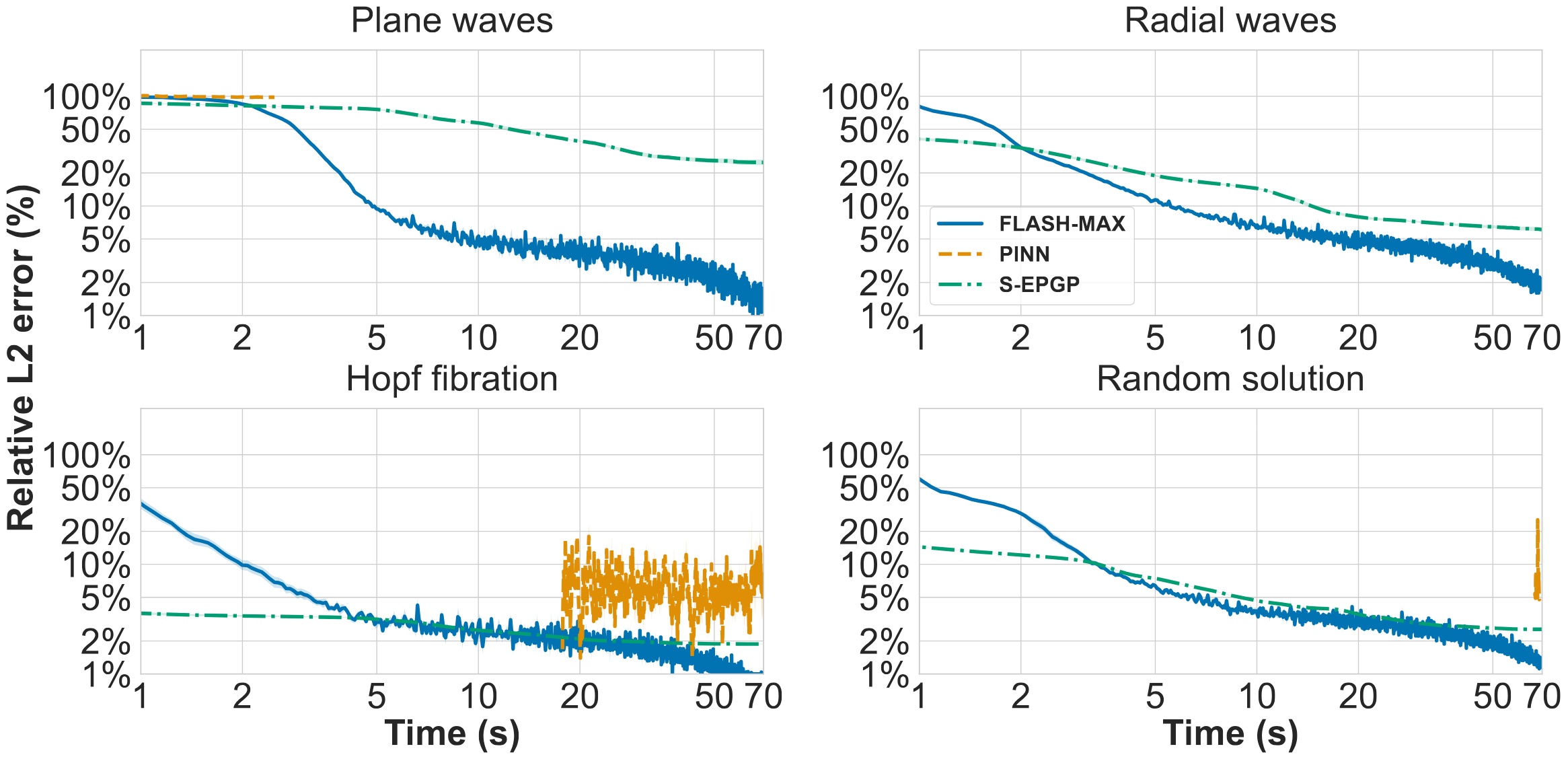
Fast-Learning Accurate Solver for the Homogeneous MAXwell equations (FLASH-MAX)
With frequencies $\mathbf{z}_{ijk}=(\textcolor{#0073e6}{z_{ijk0}},\textcolor{#b51963}{z_{ijk1},z_{ijk2},z_{ijk3}})\in \mathbb{R}^4$ s.t. $\textcolor{#0073e6}{z_{ijk0}=j\sqrt{\textcolor{#b51963}{z_{ijk1}}^2+\textcolor{#b51963}{z_{ijk2}}^2+\textcolor{#b51963}{z_{ijk3}}^2}}$,
biases $b_{ijk}\in\mathbb{R}$, Noetherian multipliers $B_{i}\colon \R^4 \to \R^6$, and $\sigma=\tanh$.
Universal approximation Theorem for Maxwell's equations
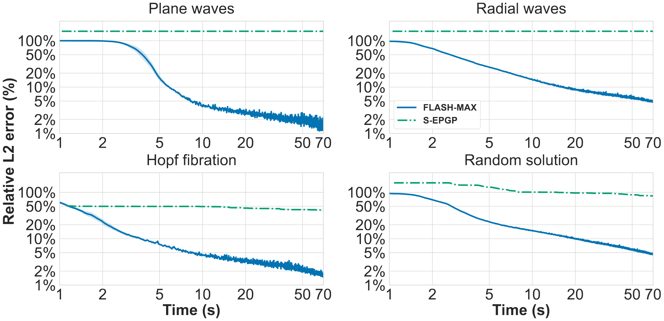
FLASH-MAX: Performance on a Time Budget
BC setup
IC setup
Conclusion
- Data structure for functions
- in computer algebra
- to model data
- with optimal control strategies
- Probability, functional analysis $\hookrightarrow$ algebra
- Fully algorithmic
- No approximations $\Rightarrow$ exact solutions
- Compatible with standard GP/NN techniques
- GPs: Very little data necessary, Bayesian UQ
- NNs: High speed
- Works well on inverse problems and control
\[ \frac{\partial^2 u}{\partial t^2} = \frac{\partial^2 u}{\partial x^2} + \frac{\partial^2 u}{\partial y^2} \]
Conclusion
\[ \frac{\partial^2 u}{\partial t^2} = \frac{\partial^2 u}{\partial x^2} + \frac{\partial^2 u}{\partial y^2} \]
Open Problems
- Increase TRL >3
- Highly accurate neural network
- Faster GPs
- Neural networks without homogeneity
- Deep neural networks
- Uncertainty quantification, active learning
- Many more...
Conclusion
Thank you for your attention!
Literature
- arXiv:2605.20514
- arXiv:2511.04518 (FLAIRS 2026)
- arXiv:2502.04276 (SSSC 2025)
- arXiv:2411.16663
- arXiv:2212.14319 (ICML oral 2023)
- arXiv:2208.12515 (NeurIPS 2022)
- arXiv:2205.03185 (CASC 2022)
- arXiv:2002.00818 (AISTATS 2021)
- arXiv:1801.09197 (NeurIPS 2018)
\[ \frac{\partial^2 u}{\partial t^2} = \frac{\partial^2 u}{\partial x^2} + \frac{\partial^2 u}{\partial y^2} \]